Display 3D terrain of the Kanto region using satellite data & Python

Let’s use free data and Python to create a 3D display of the terrain around the Kanto region in Japan.

This post utilizes NASA’s SRTM (Shuttle Radar Topography Mission) data to create a 3D model with Python.

Environment

• Ubuntu 22.04
• Python 3.10.4

Getting the data

SRTM data is free terrain data provided by NASA.

Get SRTM data from USGS EarthExplorer

1. Go to USGS EarthExplorer

Visit USGS EarthExplorer using this link:

EarthExplorer

2. Create an account

To download data, you need an account on USGS EarthExplorer. Create one here: https://ers.cr.usgs.gov/register/

3. Choose a region and dataset

On the main page of EarthExplorer, you can search for data by typing in latitude and longitude coordinates or place names in the search box. Once you have identified the area for which you would like to obtain data, you can specify it on the map by clicking on it, and then proceed with the search for data.

set area

After specifying the area, click on the ‘Data Sets’ button, and then expand the ‘Digital Elevation’ category. From there, select ‘SRTM’ and choose ‘SRTM 1 Arc-Second Global’.

4. Download the data

Click the “Results” tab, and find the right dataset from the list.

For the purpose of comparison, we will download three datasets, as follows:

1. Data including Tokyo
2. Data of the sea on the south side of Kanto
3. Data including Mount Fuji

Click the download icon to download the data files (GeoTIFF files).

The red frame in the image is manually plotted for the search. The brown and purple areas are the downloadable data ranges.

Data including Tokyo

Data of the sea on the south side of Kanto

Data including Mount Fuji

Installing Python libraries

Use the following Python libraries:

• rasterio: for reading terrain data
• numpy: for data processing
• matplotlib: for 3D plotting

Install them like this:

pip install rasterio numpy matplotlib

Implementation

I will now proceed to implement a function that creates and displays a 3D model using the downloaded SRTM data. Please note that the following instructions assume that you are using Jupyter.

import rasterio
import numpy as np
import matplotlib.pyplot as plt
from mpl_toolkits.mplot3d import Axes3D

# Function to read SRTM data
def read_elevation_data(file_path):
    with rasterio.open(file_path) as src:
        elevation_data = src.read(1)
        elevation_data = elevation_data.astype(np.float32)
        elevation_data[elevation_data < 0] = np.nan
    return elevation_data

# Function to 3D plot SRTM data
def plot_elevation_data(elevation_data_list):
    fig = plt.figure(figsize=(20, 8))

    for i, elevation_data in enumerate(elevation_data_list):
        ax = fig.add_subplot(1, len(elevation_data_list), i+1, projection="3d")
        x = np.arange(0, elevation_data.shape[1], 1)
        y = np.arange(0, elevation_data.shape[0], 1)
        x, y = np.meshgrid(x, y)
        ax.plot_surface(x, y, elevation_data, cmap="terrain")

        # Display axis names for east-west and north-south
        ax.set_xlabel('west --- east')
        ax.set_ylabel('south --- north')
        ax.set_zlabel('height [m]')

        # Fix the maximum height axis value at 3000
        ax.set_zlim(0, 3000)

    plt.show()

Drawing

Please save the SRTM data in the same directory as the Python script.

Now, let's try displaying download files in 3D.

file_paths = ["./n35_e139_1arc_v3.tif",
              "./n34_e139_1arc_v3.tif",
              "./n35_e138_1arc_v3.tif"]

elevation_data_list = [read_elevation_data(file_path) for file_path in file_paths]
plot_elevation_data(elevation_data_list)

The result will look like this:

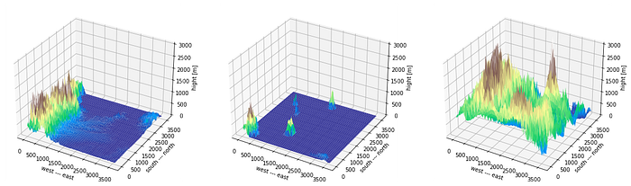
The leftmost result is the Kanto Plain, including Tokyo. Around Tokyo is shown in blue and isalmost flat. The west side is raised, showing the mountains west of Kanto.

The middle result is the sea on the south side of Kanto. You can see some islands rising, but otherwise, it’s the sea, so it’s blue and completely flat.

The rightmost result is the area around Mount Fuji. You can see that it’s mostly mountainous and has significant elevation changes.

Summary

Using satellite data and Python, we can visualize the height information of the Earth.

The SRTM data we used this time is a type of Digital Elevation Model (DEM) data. DEM data represents the terrain and elevation of the Earth, and it’s a dataset with elevation values arranged in a grid.

Since we used free data this time, the resolution is rough, and we couldn’t get detailed information. However, by using higher-resolution satellite data (probably paid), you can get more detailed height information.

This DEM data is used in various fields such as:

• Terrain analysis: Used to understand terrain features and changes and caliculate terrain elements such as slope and undulation.
• Flood risk assessment: Used to simulate flood-prone areas and inundation ranges, and plan disaster prevention measures and evacuation plans.
• Agriculture and land use: Analyze the distribution of soil and water resources and carry out land use planning and management for farmland, forests, and other areas.
• Transportation and infrastructure planning: Used to determine optimal routes and locations for infrastructure construction such as roads, railways, and dams.

In addition, we used matplotlib to visualize DEM data this time, but if you want to visualize it more interactively, there are libraries like plotly and PyVista. However, please note that handling large satellite data requires a certain level of machine specifications.

https://plotly.com/python/

https://pyvista.github.io/pyvista-docs-dev-ja/